
|
Fast and reliable calibration of solid substrate fermentation kinetic models using advanced non-linear programming techniques M. Macarena
Araya Juan J. Arrieta J. Ricardo
Pérez-Correa* Lorenz T.
Biegler Héctor Jorquera Webpage: http://www.ing.puc.cl *Corresponding author Financial support: Projects FONDECYT 1030325 and 7040084. Keywords: dynamic models, Gibberella fujikuroi, Gibberellic acid, nonlinear models, parameter estimation, secondary metabolites, solid substrate cultivation.
Calibration of mechanistic kinetic models describing microorganism growth and secondary metabolite production on solid substrates is difficult due to model complexity given the sheer number of parameters needing to be estimated and violation of standard conditions of numerical regularity. We show how advanced non-linear programming techniques can be applied to achieve fast and reliable calibration of a complex kinetic model describing growth of Gibberella fujikuroi and production of gibberellic acid on an inert solid support in glass columns. Experimental culture data was obtained under different temperature and water activity conditions. Model differential equations were discretized using orthogonal collocations on finite elements while model calibration was formulated as a simultaneous solution/optimization problem. A special purpose optimization code (IPOPT) was used to solve the resulting large-scale non-linear program. Convergence proved much faster and a better fitting model was achieved in comparison with the standard sequential solution/optimization approach. Furthermore, statistical analysis showed that most parameter estimates were reliable and accurate.
Solid substrate fermentation (SSF) can be defined as the cultivation of microorganisms on solid substrates devoid of or deficient in free water (Pandey, 2003). SSF has several advantages (Hölker and Lenz, 2005) over more conventional submerged fermentation, and many promising lab-scale SSF processes are periodically reported in the literature (John et al. 2006; Krasniewski et al. 2006; Lechner and Papinutti, 2006; Sabu et al. 2006). Unfortunately, very few of these processes enter commercial production (Hölker and Lenz, 2005) due to the magnitude of the technical difficulties in operating and optimizing large scale SSF bioreactors. Since modern process control and optimization engineering techniques are model based, mathematical modelling should significantly improve the chances of successfully transforming an SSF process from laboratory to commercial production. Nevertheless, a number of factors make modelling SSF processes particularly trying: the absence of reliable on-line measurements of relevant cultivation variables (like biomass and nutrient concentration) and the systems inherent complexity, considering that microorganism interaction with the environment and its growth and production kinetics are still not well understood on a micro scale (Mitchell et al. 2004). In addition, the more useful mechanistic dynamic models proposed are highly complex and have many parameters that need to be estimated from extensive good quality experimental data. Acquiring such data is costly and time consuming and yet, even when this data is available, attaining reliable parameter estimates is far from trivial (Gelmi et al. 2002). Therefore, in most current SSF lab-scale studies that include modelling, only simple black box or empirical kinetics models are used (Machado et al. 2004; Corona et al. 2005; Jian et al. 2005). However, these models can only reproduce process behaviour encountered in controlled conditions that are never found in large scale SSF bioreactors and, as such, more often than not commercial production yields are disappointingly low compared to lab-scale performance. Parameters in dynamic fermentation models are commonly estimated using the sequential solution/optimization (SeqSO) procedure (Rivera et al. 2006). Though simple, this procedure may be severely limited when fitting complex models with many parameters or constraints that violate standard numerical regularity conditions, as is the case of more mechanistic SSF kinetic models. A high degree of heuristics is therefore required to overcome the methods slow convergence and unreliable estimation (Gelmi et al. 2002). Alternatively, the simultaneous solution/optimization (SimSO) approach (Biegler et al. 2002) is fast, robust and reliable, and have shown its suitability for fitting a variety of complex dynamic models. In this work a SimSO procedure is developed to estimate model parameters in an SSF kinetic model and the results obtained are compared, in terms of fit quality and numerical performance, with those obtained with the commonly used SeqSO approach. The SimSO procedure developed was coded in AMPL and the resulting non-linear program (NLP) was solved using IPOPT (Biegler et al. 2002), a robust interior point NLP solver specially designed for large scale optimization problems. First, the model is described in brief and calibration details are provided. Then, results are shown and discussed, and finally the main conclusions of this work are presented. We have used a slightly modified version of the lumped parameter model proposed in (Gelmi et al. 2002) to describe cultivation in glass columns of Gibberella fujikuroi grown on an inert support (Amberlite IRA-900), urea and starch. The main assumptions of the model are:
Oxygen mass transfer resistance is negligible. Next, we present a brief description of the model. The total amount of measurable dry biomass (Xtot) considers active and inactive fungi and is expressed on a dry total mass basis (kgd.b.),
Assuming a first order death rate, the active biomass (X) is described by,
Here, μ and KD represent the specific growth rate and the specific death rate, respectively. The model assumes that urea, U, is degraded to assimilable nitrogen, NI, following zero order kinetics and that Gibberella fujikuroi uses this nutrient for biomass growth,
As this equation does not satisfy standard numerical regularity conditions we replaced equation (3) with the smooth approximation,
which is also used in the nitrogen balance below (5); ε is a small number. The concentration of assimilable nitrogen is given by,
In these equations k is the conversion rate from urea to assimilable nitrogen, 0.47 corresponds to urea nitrogen content and YX/Ni is the mass yield between biomass and assimilable nitrogen. The microorganism consumes starch for growth and maintenance,
The differential equations for CO2 production and O2 consumption rates include two terms, one associated with growth and the other with maintenance,
where YX/CO2 and YX/O2 are the mass yield coefficients between biomass and respiratory gases. GA3 net production rate includes a growth associated term with nitrogen inhibition, β, and a first order degradation rate,
The specific growth rate, μ, is modelled using Monods expression with assimilable nitrogen the limiting nutrient,
Here, μM is the maximum specific growth rate and kN is the substrate inhibition constant. A substrate inhibition expression describes the specific GA3 production rate,
where βM is the maximum specific GA3 production rate and ki is the associated substrate inhibition constant. The above model was calibrated in four culture conditions, i)
Temperature = Further details regarding the experimental set up and the above model are available elsewhere (Gelmi et al. 2000; Gelmi et al. 2002). We
have applied the simultaneous (SimSO) approach to solve the parameter
estimation problem. The set of differential equations, A differential variable is approximated as a polynomial within a finite element, on a monomial basis (Rice and Duong, 1995).
where
yi-1 is the value of the differential variable at
the beginning of element i, HD(i) is the length of element
i, dy/dtq,i is the value of the derivative in
element i at the collocation point q, ncol is the
number of collocation points
Where δq,r is the Kronecker delta
and lq(x) is the basis function for a Lagrange polynomial of order ncol, i.e.,
We have used 69 finite elements and Radau points with two internal collocation points per finite element, since this configuration achieves a good compromise between precision and efficiency and it is easy to add constraints at the end of each finite element (Rice and Duong, 1995). Integrating equation [15] with Radau points (T1 = 0.1550625; T2 = 0.6449948; T3 = 1), and ti,q = ti-1 + HD(i)·Tq, leads to values for the polynomial coefficients, W(ti,q).
with
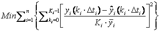
The system [15] approximates the differential variable over the respective finite element. To solve the differential equations over the entire time domain, we expand these equations for each finite element and collocation point. This large set of nonlinear algebraic equations represents a high-order implicit Runge-Kutta (IRK) approximation to the differential equations. The model parameters were estimated by weighted least squares,
Subject to,
where
n is the number of measured variables and Ki,
Δti, ŷi and y
are the number of measured values, the sampling interval, the solution
of the differential equation and the normalization value for variable
yi, respectively. The vector of estimated parameters
is represented by Because parameter k appears only in equations (3-5), and has little influence on the remaining state variables, it is estimated separately and can be obtained directly from the urea consumption curve. In addition, it was also verified that parameters mM and kN in equation [9] are correlated, since many combinations of these parameter values achieved the same data fit. Thus, we obtained the values of mM from curves of the accumulated respiratory gases (Saucedo-Castañeda et al. 1994), and estimated kN using the least squares procedure described above. The values obtained of both rates (k and mM) for all cultivation conditions are given in Table 1. The vector of estimated parameters, therefore, through least squares using equations 17 and 18 is θ = (ki, kN, kP, mCO2, mO2, mS, KD, YX/CO2, YX/O2, YX/N, YX/S, βM). The resulting large scale optimization problem was solved in AMPL using IPOPT solver (Biegler et al. 2002). Results obtained with the procedure described above were compared with those obtained with the SeqSO approach, as described in Gelmi et al. (2002). Once
the optimization is carried out, the solution of (17, 18) can be formally
written as ŷ = F(
We have found that using ∆θ = 0.001 θ is sufficient to obtain accurate estimates of the Jacobian. Now, since the number (n) of experimental points is large enough (O(103)), we can use the linear approximation (Seber and Wild, 1998) to use the result:
Where
θ* is the true parameter vector, We compare our calibration results for each cultivation condition with the fit obtained using the SeqSO approach. We were specifically interested in fit quality, the performance of the optimization procedure and the value and accuracy of the estimated parameters. Cultivation
condition 1 (T = In Table 2 we can see that the SimSO estimation of the GA3 inhibition constant, ki, was highly inaccurate (large σ) yet the parameter is significant; the SimSO estimation of the GA3 degradation rate constant, kp, was unreliable (t value is almost zero). Therefore, it is pointless to compare the two methods estimation of these parameters. Other parameter estimates were reliable (t values above 2) and accurate (relatively small σ). We dont have the estimation of σ for the parameters obtained with the SeqSO calibration method. Therefore, if we assume that both methods yield the same σ it is reasonable, as a first approximation, to consider that both parameter estimates are similar when their difference is smaller than 3 times the standard deviation computed for the SimSO estimate (Wild and Seber, 2000). Then, in this cultivation condition four parameter estimates differed significantly using the two fitting methods, the Monods constant in equation [10], kN, the biomass/oxygen yield coefficient, YX/O2, the biomass/nitrogen yield coefficient, YX/N, and the maximum specific GA3 production rate, βM. We should expect therefore model simulations with both parameter sets to be similar. This supposition is supported by a marginal improvement in the objective function (equation 17) (see Table 3). Hence, the SimSO method shows only a slightly better fit for the respiratory gases (Figure 2) and the other model variables are almost indistinguishable for the two methods (not shown). For the particular conditions of cultivation 1, the main advantage of the SimSO calibration procedure is its efficiency and robustness. We started from two different guesses and achieved the same estimation parameters in less than 30 CPU s on an Athlon XP 2K PC, running Windows XP. Here, deviation errors in equation [17] were normalized by the maximum measured value. Cultivation
condition 2 (T = Under these conditions there was an unusual delay of 20 hrs in microorganism growth, which the model does not consider. Hence, calibration only included the data after 20 hrs. Estimates for ki and kP were not significant (t value below 2); most of the other parameter estimates were very significant (t above 10), as shown in Table 4. The SimSO fit presented estimated parameter values different from the SeqSO method, except for the death rate constant, KD, the biomass/nitrogen yield coefficient, YX/N, and the oxygen maintenance coefficient, mO2. Despite the differences in parameter values observed in Table 4, only oxygen consumption and GA3 production curves differed significantly in fittings with the two methods (Figure 3). Moreover, the objective function value of the SimSO calibration is just 10% lower than the SeqSO result (Table 3). Here, deviation errors in the objective function were also normalized by the maximum measured value. Since starting from two different guesses produced the same set of estimates in less than 30 sec, just like in the fitting of condition 1, the SimSO calibration procedure for this data was efficient and robust. Cultivation
condition 3 (T = Table 5 shows that under these conditions, the kP SimSO estimate was not significant. However, contrary to cultivation conditions 1 and 2, the ki estimate was significant and more accurate; at least here, contrary to cultivations 1 and 2, σ for this parameter is smaller than the estimate values allowing us to compare both methods. Again, the rest of the parameter estimates were significant and accurate. Table 5 shows that both methods yielded different estimates for all model parameters, except for the death rate constant, KD. Moreover, a much better fit was achieved with SimSO parameter values for biomass, GA3 and starch (Figure 4) that, in turn, is reflected in the sharp reduction in the objective function (Table 3). Here, again, deviation errors were normalized by the maximum measured value and optimization was started from two different initial guesses. Convergence was more difficult than for the previous cultivation conditions, requiring more iterations and CPU time (Table 3). Cultivation
condition 4 (T = Here,ki and kP estimates were not significant, while the remaining SimSO parameter estimates were accurate and significant (Table 6). Except for mCO2, YX/CO2 and YX/N, SimSO parameter estimates did not stray much from the SeqSO estimates. Nevertheless, the SimSO procedure achieved a better fit for biomass and GA3 (Figure 5), and a significantly lower objective function value (Table 3). Convergence for these conditions was the most difficult of the 4 cases, requiring a 5-fold increase in CPU time than in cultivation conditions 1 and 2 (Table 3) and twice as much as cultivation 3. We had to normalize by the average measured value in equation [17] to get convergence here, too. In
a comparison of cultivation conditions 1 and 4 only the death rate
was unaffected by temperature (Table 2 and
Table 6). The other model parameters took
on different values at the two temperatures. For instance, μM,
βM and the maintenance coefficients increased
with temperature, while the yield coefficients and kN
decreased with temperature (Table 1, Table
2 and Table 6). The net result was that
at Comparing cultivation conditions 1 and 2, we observe that, except for mS, water activity had little effect on the maintenance coefficients. Yield coefficients, μM and βM were higher for aw = 0.992, while kN and KD were lower (Table 1, Table 2 and Table 4). The net result was that for aw = 0.992 around 30% more biomass and twice as much GA3 were produced (results not shown). Comparing cultivations 3 and 4, on the other hand, we observe that for aw = 0.985 the death rate was unaffected, kN, βM and maintenance coefficients were higher, while the yield coefficients and μM were lower (Table 1, Table 5 and Table 6). Therefore, for aw = 0.985 less biomass and a little more GA3 were obtained (results not shown). Overall, estimation of GA3 kinetic parameters proved awkward. Estimations of kp were unreliable and close to zero for all cultivation conditions, and indicates that GA3 degradation in these experiments was most probably negligible. Moreover, estimations of ki were unreliable or inaccurate in almost all instances. GA3 is a secondary metabolite that Gibberella starts producing when available nitrogen in the medium is almost exhausted. Therefore, many measurements close to the point of nitrogen exhaustion are required to obtain accurate estimations of ki. In the range studied, we also verified that βM increases with temperature yet it decreases with water activity. Regarding variations of growth kinetic parameters, we found the death rate was unaffected by temperature and reached a maximum for aw = 0.999. In addition, μM increased with temperature and water activity, while kN decreased with temperature and it appeared to reach a minimum at aw = 0.992. Maintenance coefficients increased with temperature and took their highest values at aw = 0.985. In turn, yield coefficients decreased with temperature and appeared to reach their maximum at aw = 0.992. The importance of this work is the significant reduction in convergence time the SimSO approach achieved. As a consequence it drastically simplified the parameter estimation problem. A typical calibration with the SeqSO approach, as described in Gelmi et al. (2002), required many runs of the optimization program, each taking several hours to converge and requiring a high degree of heuristics and, in all, the entire SeqSO procedure took over a week to complete. Another important consideration is that for most conditions the SimSO calibration strategy achieved a significantly better fit for biomass, GA3 and oxygen consumption. The method used here is a valuable tool and should contribute appreciably to the development and testing of complex SSF mechanistic models. The authors thank Alex Crawford for his assistance in improving the style of the text. BIEGLER, Lorenz T.; CERVANTES, Arturo M. and WÄCHTER, Andreas. Advances in simultaneous strategies for dynamic process optimization. Chemical Engineering Science, February 2002, vol. 57, no. 4, p. 575-593. [CrossRef] HÖLKER, Udo and LENZ, Jürgen. Solid-state fermentation - are there any biotechnological advantages? Current Opinion in Microbiology, June 2005, vol. 8, no. 3, p. 301-306. [CrossRef] JIAN, Xu; SHOUWEN, Chen and ZINIU, Yu. Optimization of process parameters for poly γ glutamate production under solid state fermentation from Bacillus subtilis CCTCC202048. Process Biochemistry, September 2005, vol. 40, no. 9, p. 3075-3081. [CrossRef] JOHN, Rojan P.; NAMPOOTHIRI, K. Madhavan and PANDEY, Ashok. Solid-state fermentation for L-lactic acid production from agro wastes using Lactobacillus delbrueckii. Process Biochemistry, April 2006, vol. 41, no. 4, p. 759-763. [CrossRef] KRASNIEWSKI, Isabelle; MOLIMARD, Pascal; FERON, Gilles; VERGOIGNAN, Catherine; DURAND, Alain; CAVIN, Jean-François and COTTON, Pascale. Impact of solid medium composition on the conidiation in Penicillium Camemberti. Process Biochemistry, June 2006, vol. 41, no. 6, p. 1318-1324. [CrossRef] LECHNER, B.E. and PAPINUTTI, V.L. Production of lignocellulosic enzymes during growth and fruiting of the edible fungus Lentinus tigrinus on wheat straw. Process Biochemistry, March 2006, vol. 41, no. 3, p. 594-598. [CrossRef] MACHADO, Cristina M.M.; OISHI, Bruno O.; PANDEY, Ashok and SOCCOL, Carlos R. Kinetics of Gibberella fujikuroi growth and gibberellic acid production by solid-state fermentation in a packed-bed column bioreactor. Biotechnology Progress, September 2004, vol. 20, no. 5, p. 1449-1453. [CrossRef] MITCHELL, David A.; VON MEIEN, Oscar F.; KRIEGER, Nadia and DALSENTER, Farah Diba H. A review of recent developments in modeling of microbial growth kinetics and intraparticle phenomena in solid-state fermentation. Biochemical Engineering Journal, January 2004, vol. 17, no. 1, p. 15-26. [CrossRef] PANDEY, Ashok. Solid-state fermentation. Biochemical Engineering Journal, March 2003, vol. 13, no. 2-3, p. 81-84. [CrossRef] RICE,
Richard G. and DUONG, Do D. Applied mathematics and modeling
for chemical engineers. RIVERA, Elmer Copa; COSTA, Aline C.; ATALA, Daniel I.P.; MAUGERI, Francisco; WOLF MACIEL, Maria R. and MACIEL FILHO, Rubens. Evaluation of optimization techniques for parameter estimation: Application to ethanol fermentation considering the effect of temperature. Process Biochemistry, July 2006, vol. 41, no. 7, p. 1682-1687. [CrossRef] SABU, A.; AUGUR, C.; SWATI, C. and PANDEY, Ashok. Tannase production by Lactobacillus sp. ASR-S1 under solid-state fermentation. Process Biochemistry, March 2006, vol. 41, no. 3, p. 575-580. [CrossRef] SAUCEDO-CASTAÑEDA, G.; TREJO-HERNÁNDEZ, M.R.; LONSANE, B.K.; NAVARRO, J.M.; ROUSSOS, S.; DUFOUR, D. and RAIMBAULT, M. On-line automated monitoring and control systems for CO2 and O2 in aerobic and anaerobic solid-state fermentations. Process Biochemistry, 1994, vol. 29, no. 1, p. 13-24. [CrossRef] SEBER,
George A.F. and WILD, C.J. Nonlinear Regression. WILD,
C.J and SEBER, George A.F. Chance encounters: A first course
in data analysis and inference. Note: Electronic Journal of Biotechnology is not responsible if on-line references cited on manuscripts are not available any more after the date of publication. |
|
|
 [4]
[4]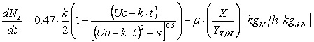 [5]
[5] [6]
[6]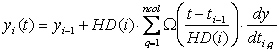 [12]
[12] [14]
[14]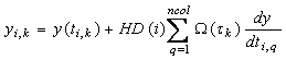 [16]
[16]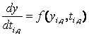
 [17]
[17] [18]
[18]